| nlfff_cat, | input,catfile,dir |
| nlfff_init, | input,catfile,it,run,dir,savefile |
| nlfff_hmi, | dir,savefile,test,datadir |
| nlfff_aia, | dir,savefile,test,wave_,datadir |
| nlfff_fov, | dir,savefile,test,datadir |
| nlfff_magn, | dir,savefile,test,datadir |
| nlfff_tracing, | dir,savefile,test,datadir |
| nlfff_fit, | dir,savefile,test |
| nlfff_field, | dir,savefile,test |
| nlfff_cube, | dir,savefile,test,cube |
| nlfff_merit, | dir,savefile,test |
| nlfff_energy, | dir,savefile,test |
| nlfff_disp, | dir,catfile,iflare,it,run,io |
| nlfff_disp2, | dir,catfile,iflare,it,run,overlay,ngrid,bmin |
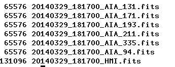
The task NLFFF_CAT generates a catalog "event_tutorial_runZ.txt" with NT=duration/cadence = 4500 s / 360 s = 13 time steps, defining the UT times and heliographic positions for each time step. The task NLFFF_INIT reads the time, heliographic position, and wavelengths of the requested time step IT=1 from the catalog and generates an IDL savefile with the name "20140329_181700_AIA_001_runZ.sav" for this run, in which all results will be saved. The task NLFFF_HMI reads the corresponding HMI/SDO image from the Stanford/JSOC archive, if the magnetogram file does not aready exist in the specified local directory. The HMI Fitsfile is named "20140329_181700_HMI.fits". The procedure NLFFF_AIA downloads the 6 requested AIA full-disk images from the Lockheed Martin or Stanford/JSOC archive, if the datafiles do not already exist in the specified local directory. The procedure NLFFF_IRIS reads the corresponding IRIS slit-jaw images if necessary. The data input is now complete and the work directory should contain the following data files:
If this code is not able to download the datafiles directly,
please download them from JSOC and make sure that the files are
renamed according to the naming convention used here. For this
particular example you can download the data files from the
follwing webpage:
20140329_181700_AIA_131.fits"
20140329_181700_AIA_171.fits"
20140329_181700_AIA_193.fits"
20140329_181700_AIA_211.fits"
20140329_181700_AIA_335.fits"
20140329_181700_AIA_94.fits"
20140329_181700_HMI.fits"
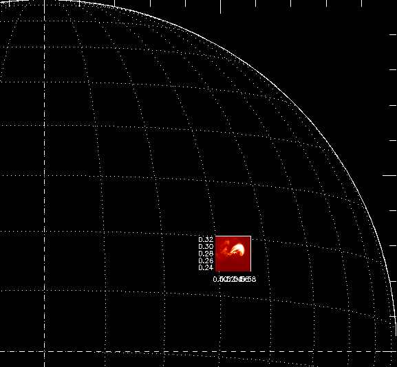
The task NLFFF_FOV extracts subimages in the specified field-of-view
with size FOV=0.3 solar radii and centered around the heliographic
position N07W30. The subimages are saved as separate FITS files and
the control display looks like this (if the parameter TEST=1 is set):
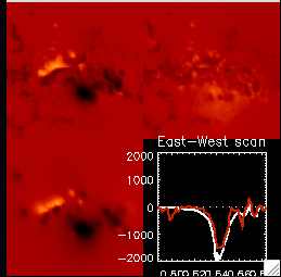
The task NLFFF_MAGN extracts the corresponding subimage from the HMI magnetogram and decovolves the line-of-sight magnetogram into the specified NMAG_P=200 potential field magnetic sources. A control display (if TEST=1 is set) is shown with the original magnetogram (top left), the decomposed model of the magnetogram (bottom left), the difference between the observed and the model diagram (top right panel), as well as an East-West scan through both the original (red curve) and model magnetogram (white curve) (bottom right panel).
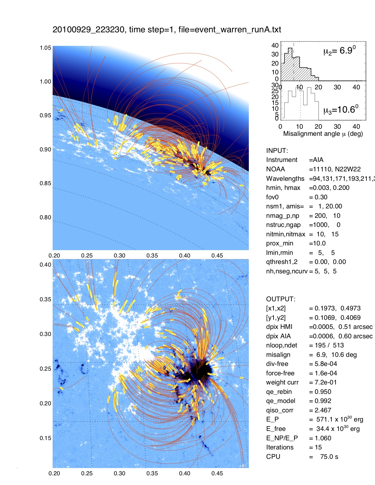
The task NLFFF_TRACING traces then in each of the 8 AIA wavelength images curvi-linear features and displays the tracings superimposed on one of the AIA images (if TEST=1 is set). The task NLFFF_FIT is then the main computation task that fits a nonlinear force-free solution to the geometry of the traced loops, by minimizing the median 3D misalignment angle. Typical computation times are about 1 minute. The task NLFFF_FIELD computes then a specific data set of modeled field lines that intersect the midpoints of the automatically traced loop segments. The procedure NLFFF_CUBE can be used to calculate an entire 3D cube of B-field vectors, if CUBE=1 is set, otherwise a minimum cube with only nz=3 bottom layers is calculated. The routine NLFFF_MERIT calculates also some figures of merit, and the task NLFFF_ENERGY integrates the non-potential and free energy over the entire computation volume. In a final step, a quick display of the results can be produced with the procedure NLFFF_DISP, which shows the obtained 3D loop trajectories and field lines from two different aspect angles (line-of-sight and 90 deg rotated to North. A postscript file is automatically produced from this display, with the filename "20140329_181700_AIA_001_runA_col.ps":
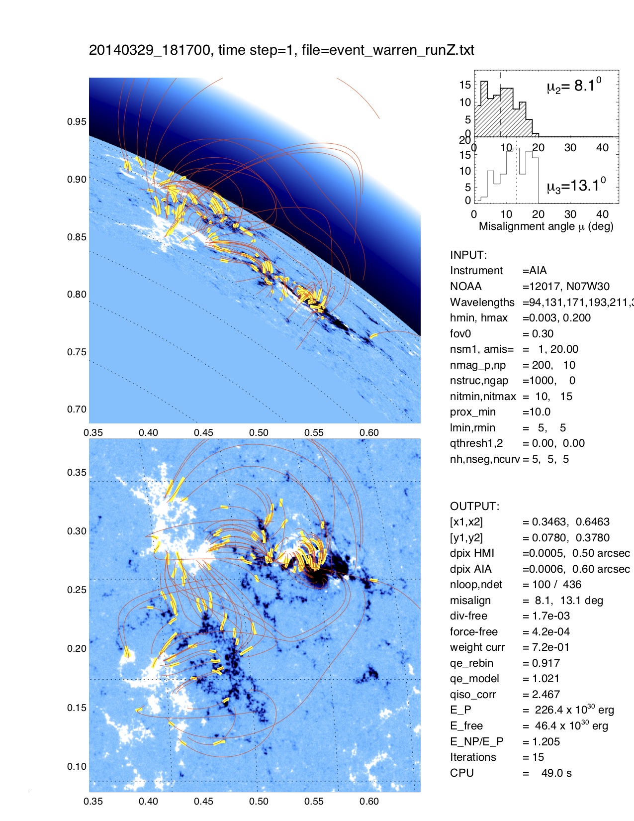
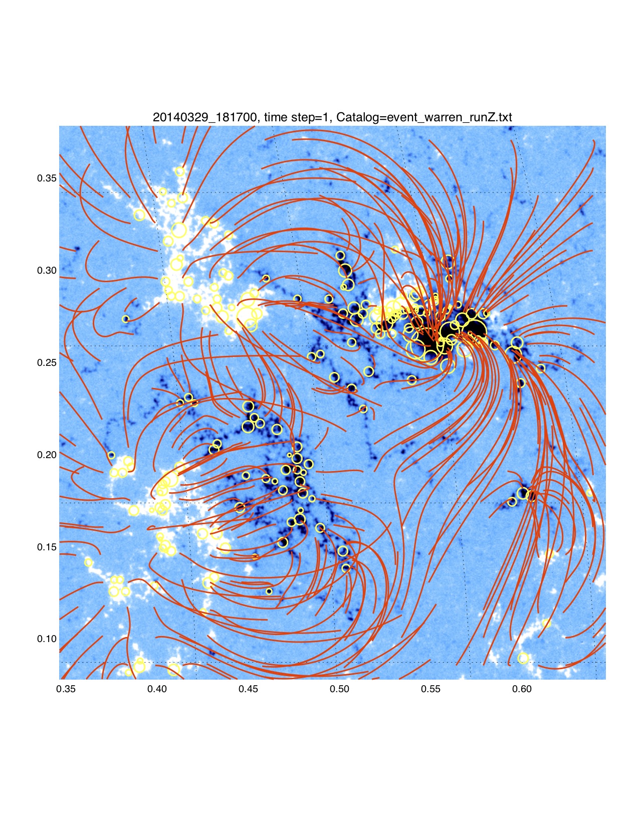
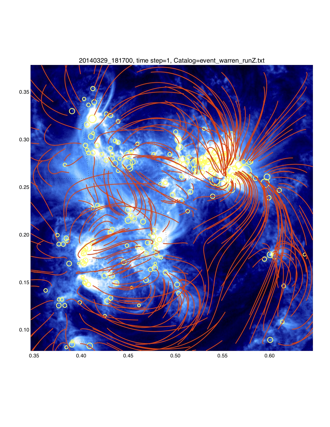
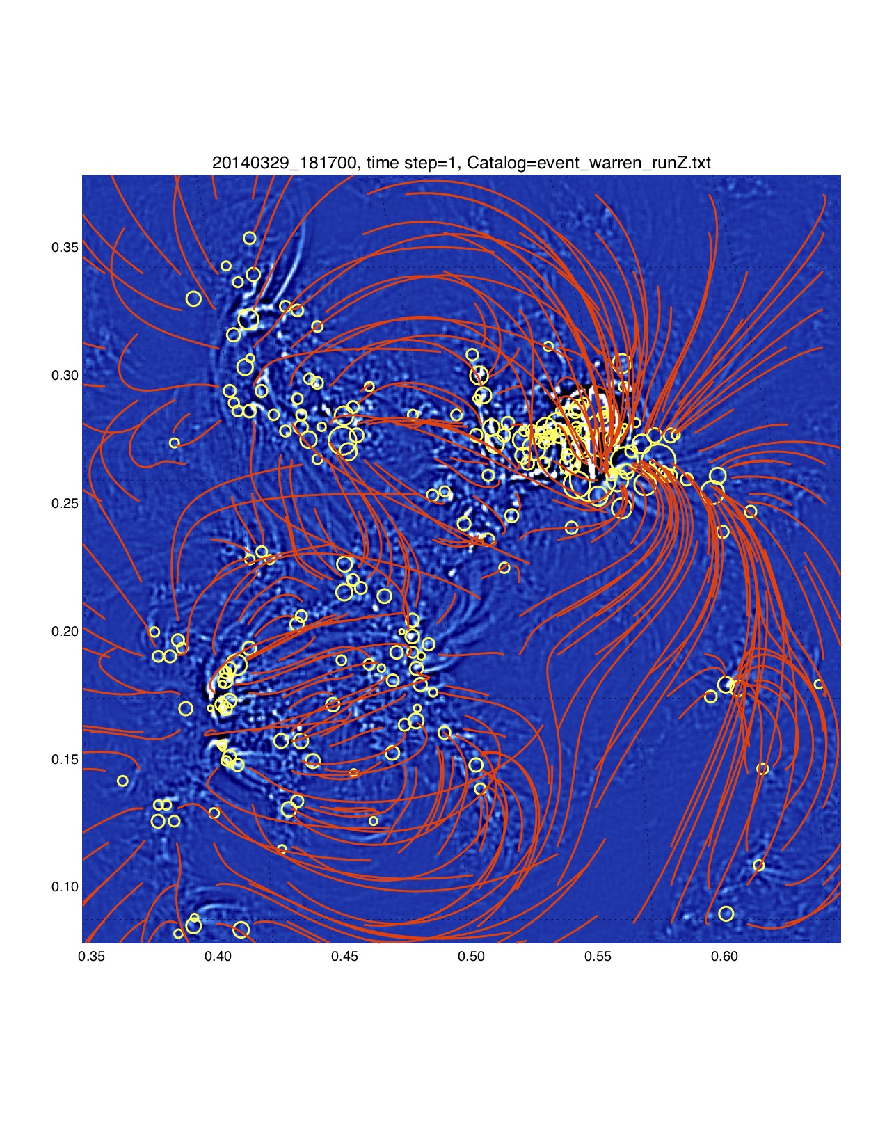
This standard plot is created with the procedure NLFFF_DISP.PRO. Other overlay plots can be created with the procedure NLFFF_DISP2.PRO, using different overlay options or field line selections. The parameter OVERLAY=0 shows the HMI magnetogram as background. The choice of OVERLAY=171 will show the 171 A EUV image as background on a logarithmic color scale, while OVERLAY=-171 (negative wavelength) which show the highpass filtered 171 A image as background. For the choice of field line selections, either the field lines that intersect the midpoints of the traced loop segments can be chosen (standard option in NLFFF_DISP and NLFFF_DISP2), or a rectangular grid of footpoints, say NGRID=2 will select footpoints in a 20 x 20 grid, with a threshold set by the minimum magnetic field strength in units of Gauss, for instance BMIN=10. The output will be stored in a postscript file with the name "20140329_181700_AIA_001_runZ2.sav'. Note that NLFFF_DISP produces a plot names *runZ_col.ps, while the NLFFF_DISP2 produces a plot with *runZ2_col.ps.
DISPLAY OVERLAYS AND FIELD LINES_______________________________________
| overlay = 0 | ;HMI magnetogram |
| ngrid = 0 | ;field lines intersecting midpoints of traced loops |
| bmin = 10 | ;(G) |
| nlfff_cat, input,catefile,dir | |
| nlfff_disp, dir,catfile,iflare,it,run | |
| nlfff_disp2, dir,catfile,iflare,it,run,overlay,ngrid,bmin,datadir | |
DISPLAY EUV IMAGE AND FIELD LINES WITH FOOTPOINT GRID____________________
| overlay = 171 | ;171 A AIA/SDO image on log scale |
| ngrid = 20 | ;field lines grid with 20 x 20 footpoints |
| bmin = 10 | ;(G) |
| nlfff_disp2, dir,catfile,iflare,it,run,overlay,ngrid,bmin | |
DISPLAY HIGHPASS-FILTERED EUV IMAGE AND FIELD LINES_______________________________________
| overlay = -171 | ;171 A AIA/SDO image highpass-filtered |
| ngrid = 20 | ;field lines grid with 20 x 20 footpoints |
| bmin = 10 | ;(G) |
| nlfff_disp2, dir,catfile,iflare,it,run,overlay,ngrid,bmin | |
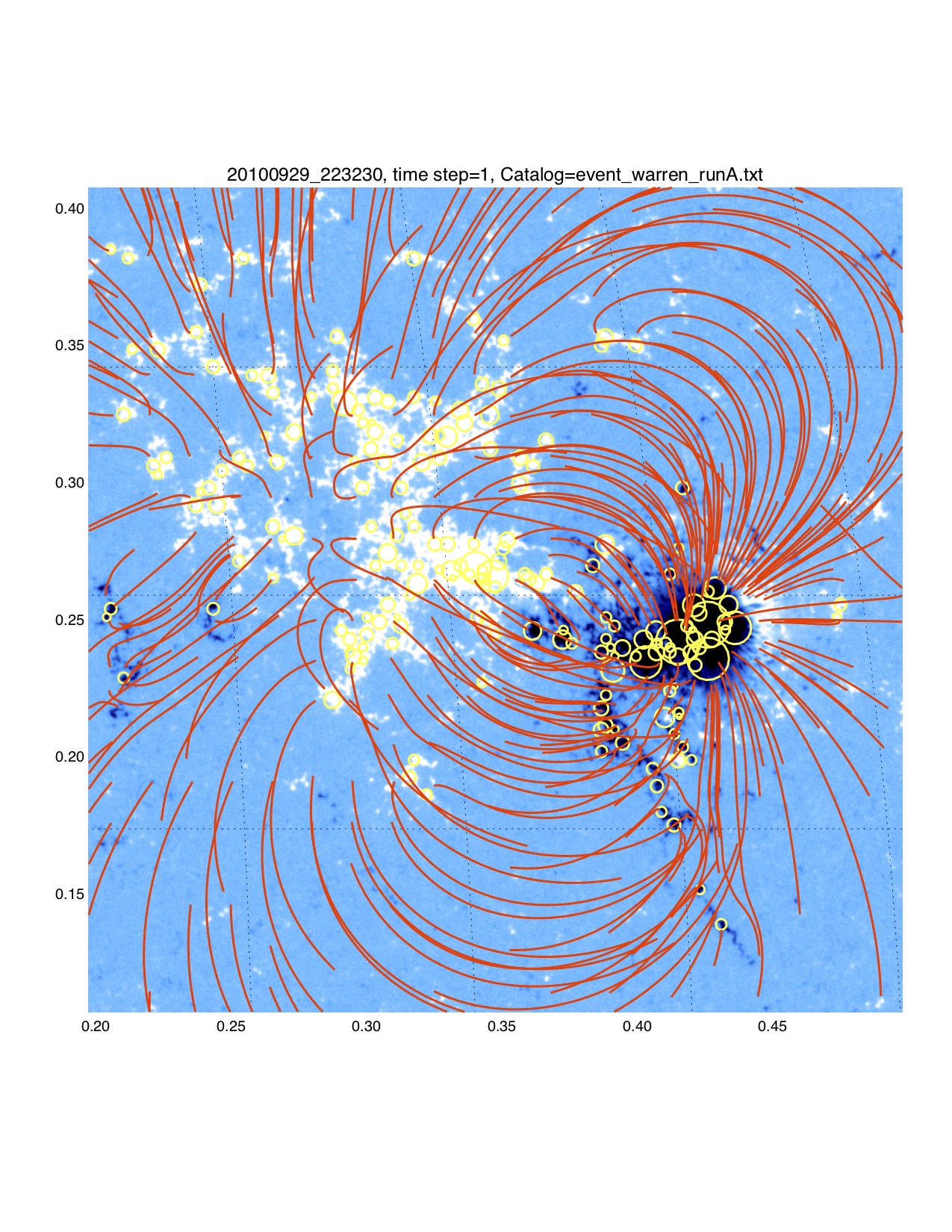
(A) Active Region NOAA 11110 observed on 2010 Sept 29
In this example we use a larger field of view (FOV=0.3 solar radii), only one wavelength INPUT.WAVE8=[0,0,171,0,0,0,0,0], a larger highpass filter NSM1=3, more magnetic sources, NMAG_P=60, NMAPG_NP=60, the largest range of acceptable misalignment angles INPUT.AMIS=90 (degrees), and a threshold of QTHRESH2=1.0 standard deviations in the filtered image.
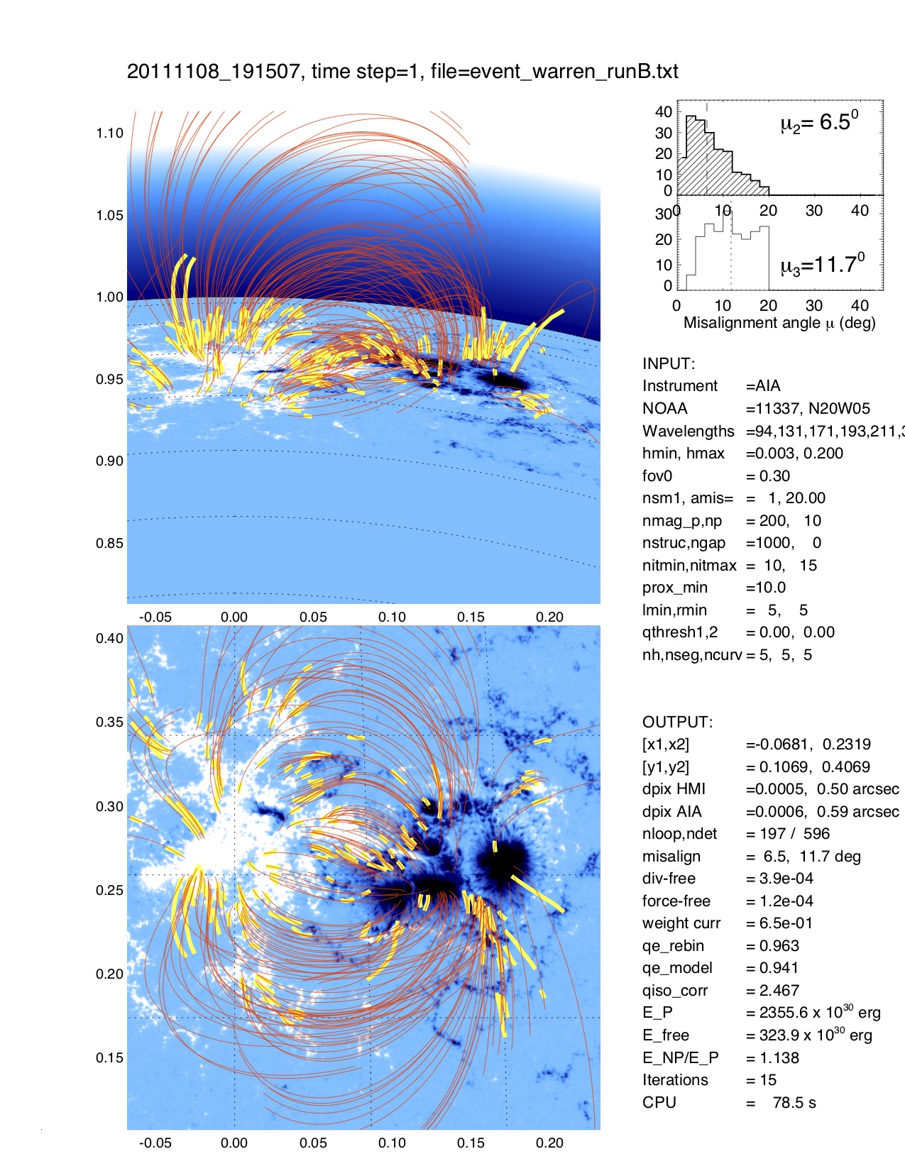
(B) Active Region NOAA 11337 observed on 2011 Nov 8

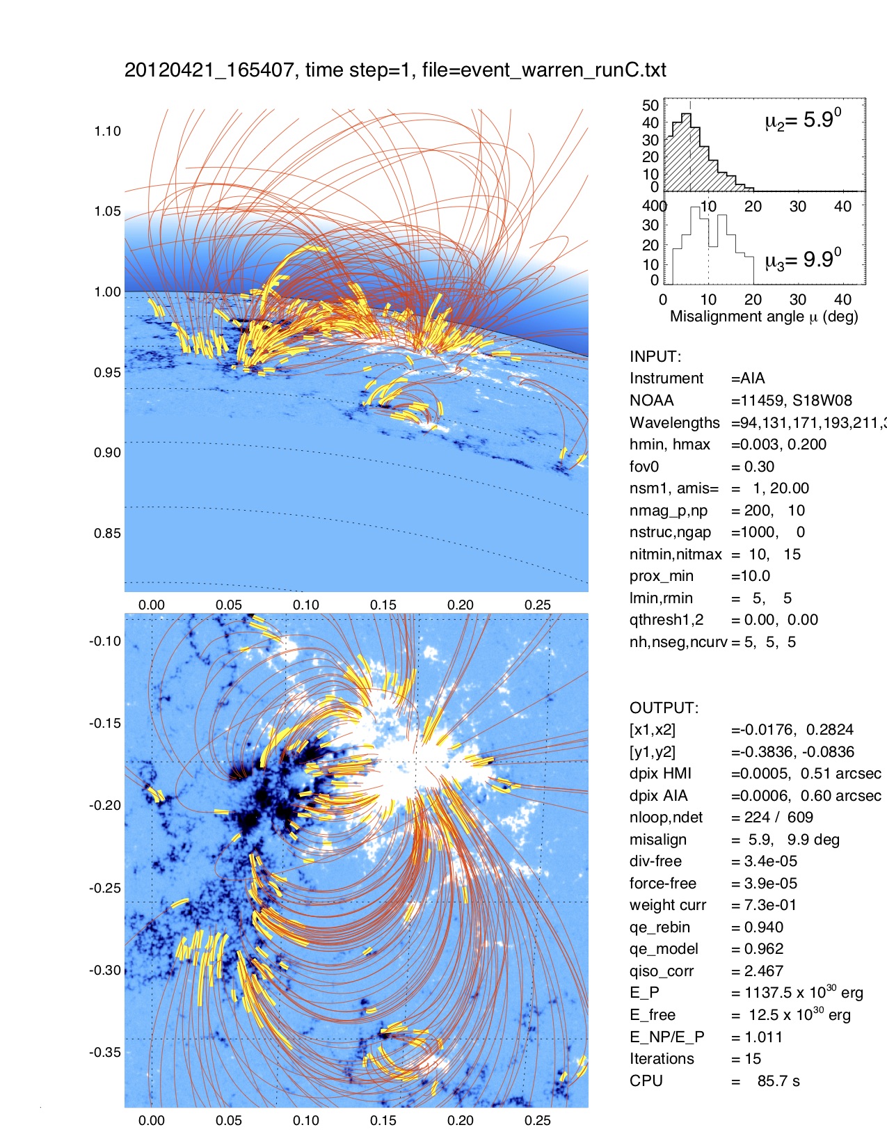
(C) Active Region NOAA 11459 observed on 2012 Apr 21

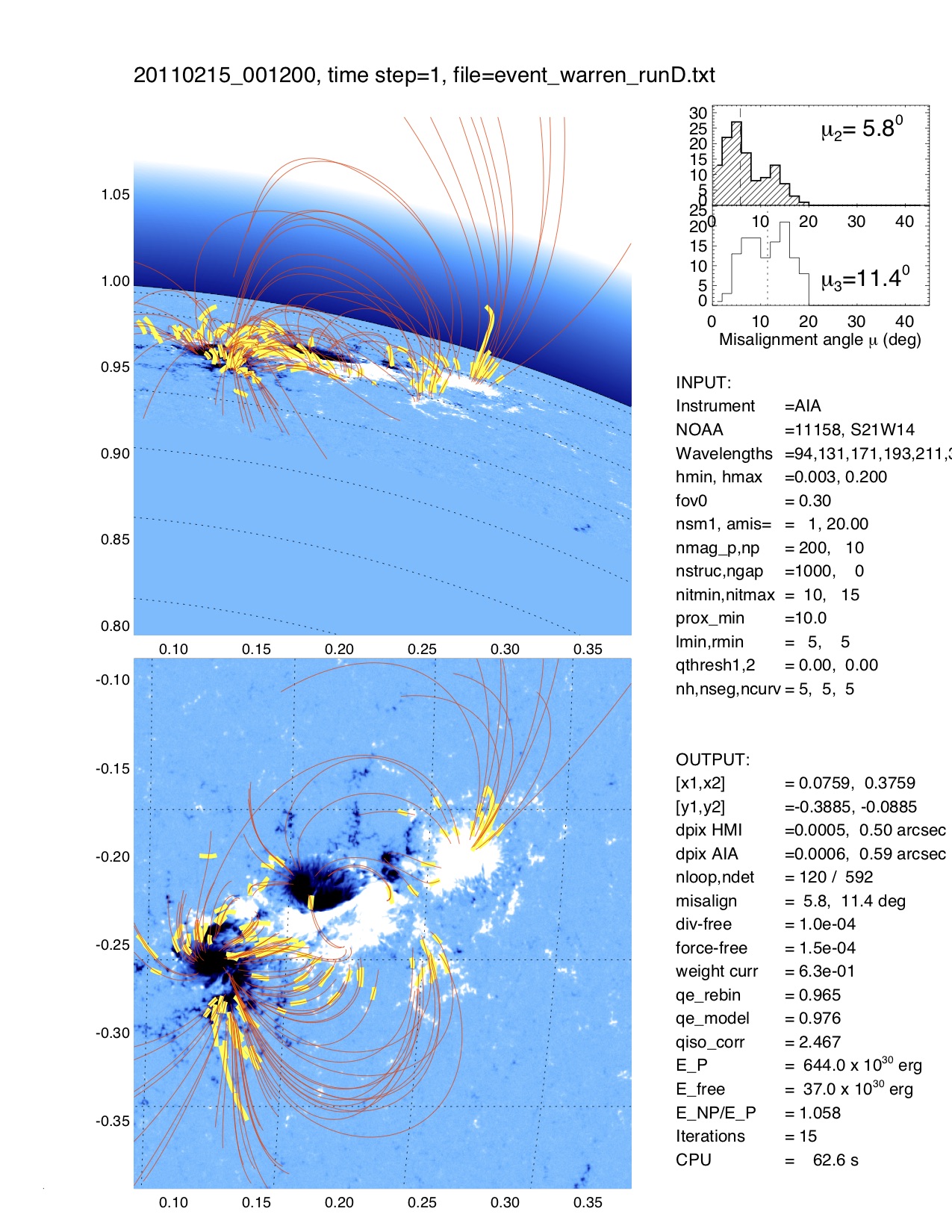
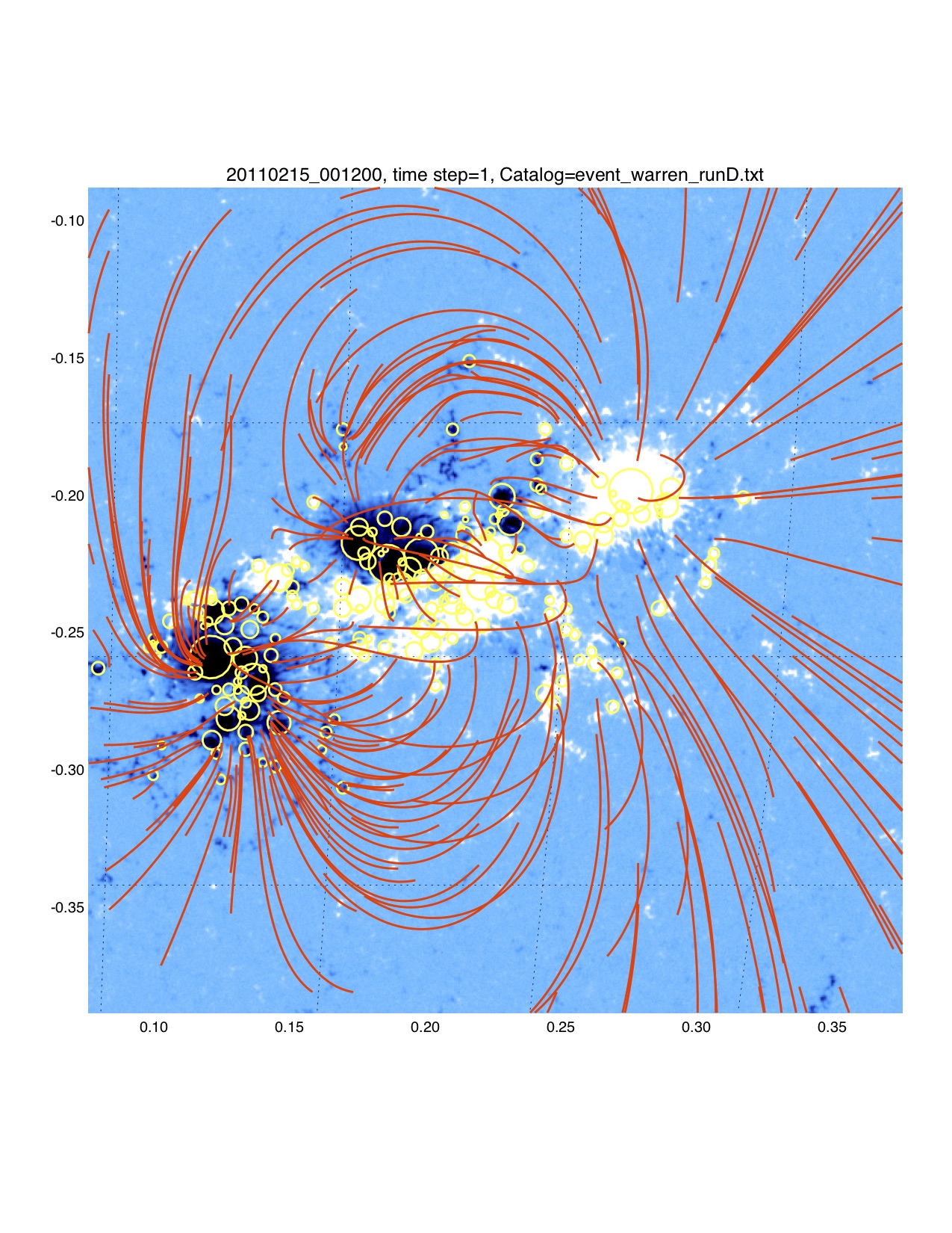
(D) Active Region NOAA 11158 observed on 2011 Feb 15
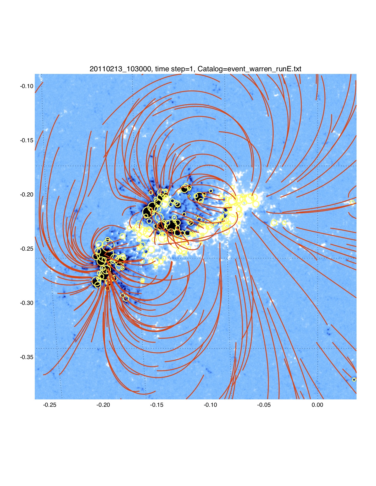
(E) Active Region NOAA 11158 observed on 2011 Feb 13

E-mail: aschwanden@lmsal.com - Markus J.Aschwanden (Lockheed Martin Solar & Astrophysics Lab.)