Aschwanden,M.J. and Tsiklauri,D.T. 2009, The Astrophysical Journal Supplement
Series Vol. 181., p. 171-185
URL1="../eprints/2009_hydroapprox.pdf"
The Hydrodynamic Evolution of Impulsively Heated Coronal Loops:
Explicit Analytical Approximations
The IDL procedures of this code should be available in SolarSoft and have the names:
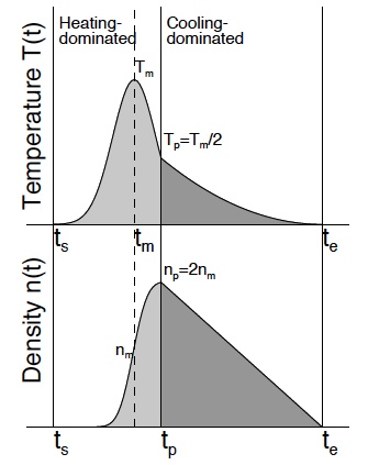
The impulsive heating function is given by a Gaussian time profile with maximum heating rate EH_m=EH(t=t_m) at time t=t_m and with a gaussian width t_heat, which is the heating time scale. The spatial heating function is characterized with the (exponential) heating scale height s_h, which is positive for footpoint heating, infinite for uniform heating, and negative for apex heating. Another parameter is the loop half length L. Everything else is dependent on these 5 input parameters. A generic diagram of the resulting time evolution of the electron density n(t) and temperature T(t) is shown in the figure above. We calculate now an example that is shown in Fig.7 of the paper quoted above, where it is also compared with an exact numerical hydrodynamic simulation (Tsiklauri et al. 2004, A&A 419, 1149):

E-mail:
aschwanden@lmsal.com -
Markus J.Aschwanden (Lockheed Martin Solar & Astrophysics Lab.)
IDL>
l = 27.5e8
; .... [cm] loop half length
s_h = -8.75e8
; .... [cm] heating scale height (positive for footpoint heating, negative for apex heating)
eh_m = 3.0/exp(l/abs(s_h))
; .... [erg cm-3 s-1] maximum heating rate (apex heating rate) OR ...
;eh_m = 7.5
; .... [erg cm-3 s-1] maximum heating rate (footpoint heating rate)
eh_bg = 1.e-8
; .... [erg cm-3 s-1] background heating rate
theat = 164
; .... [s] heating time scale (Gaussian width of EH(t)
t_m = 822
; .... [s] time of maximum heating
t=findgen(5000)
; .... [s] time array
hydro_approx1,eh_m,theat,l,s_h,t_m,t,eh_ana,te_ana,ne_ana,pe_ana,t_p,t_e,te_p,ne_p,tcond,trad,tcool,eh_bg,te_bg,ne_bg,te_avg,ne_avg,pe_avg
The time evolution of the various physical parameters is plotted with:
plot,t,eh_ana,yrange=[0,1.2*eh_m],xtitle='Time t[s]',ytitle='Heating rate EH(t)'
plot,te_ana/1.e6,yrange=[0,1.2*max(te_ana)/1.e6],xtitle='Time t[s]',ytitle='Temperature T(t) [MK]'
plot,t,ne_ana,yrange=[0,1.2*max(ne_ana)],xtitle='Time t[s]',ytitle='Electron density n(t)'
plot,alog10(ne_ana),alog10(te_ana),xtitle='Density log(n)',ytitle='Temperature log(T)',xrange=[8,12],yrange=[6,8]
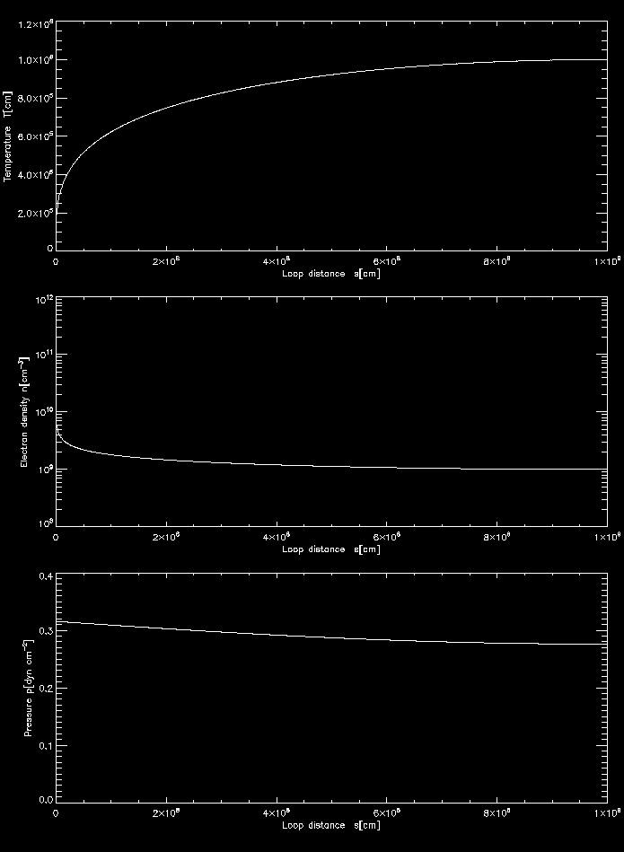
Example 2: Analytical Approximation of Spatial Hydrostatic Profiles
Is we assume that the heating time scale is sufficiently long to ensure
nearly hydrostatic equilibrium at any instant of time, we can obtain
the spatial profiles of temperature, density, and pressure with the
analytical solutions for hydrostatic equilibrium. Here an example:
l = 1.0e9
; .... [cm] loop half length
s_h = l*100
; .... [cm] heating scale height (uniform case: s_h>>l)
te_l = 1.0e6
; .... [K] loop top temperature
ne_l = 1.0e9
; .... [K] loop top electron density
th = 0
; .... [deg] loop plane inclination angle
ns = 1000
; .... number of loop position
hydro_approx2,l,s_h,te_l,ne_l,th,ns,s,te_s,ne_s,p_s
plot,s,te_s
plot_io,s,ne_s
plot,s,p_s