Automated Detection of Coronal Loops (Tutorial)

Code: Oriented Coronal CUrved Loop Tracing (OCCULT-2)

This tutorial is intended for SolarSoftWare (SSW) users who want to detect curvi-linear structures with large curvature radii in an image, such as coronal loops, but it might work also for other curved features (filaments, prominences, plumes, streamers, CME leading edges, sunspot penumbral fibres, etc.). The software is mostly trained on TRACE images, but should also work for other EUV or soft X-rays images, such as from SOHO/EIT, STEREO/EUVI, Hinode/XRT, SDO/AIA. The numeric code OCCULT is described in the paper:

A Code for Automated Tracing of Coronal Loops Approaching Visual Perception (OCCULT-1 code)
by M.J.Aschwanden (2010), Solar Physics 262, 399-423.
../eprints/2010_autoloop.pdf"

Optimization of Curvi-Linear Tracing Applied to Solar Physics and Biophysics (OCCULT-2 code)
by M.J.Aschwanden, B. DePontieu, and E. Katrukha (2013), Entropy, Special Issue on Advanced Signal Processing in Heliophysics (in press).
../eprints/2013_entropy.pdf"

The IDL routines are available in the package $/SSW/package/mjastereo/idl/, which are automatically included in the IDL path with the command IDL>setenv SSW_INSTR "stereo".

(1) TRACE Data Examples

The following example uses the latest version of the OCCULT-2 code (Aschwanden, DePontieu, and Katrukha 2013), which calls the IDL routine LOOPTRACING_AUTO4.PRO from the user-contributed SSW library, which we recommend instead of using the earlier version LOOPTRACING_AUTO.PRO, *AUTO2.PRO or *AUTO3.PRO (with a slightly different input format). We read a 2-D image from a FITS-file named 'TRACE_19980519.fits, which is used as input IMAGE1 for the IDL procedure LOOPTRACING_AUTO4.PRO. In addition there are 8 control parameters that can be set by the user and are passed to the routine with the array PARA=FLTARR(8). The output of the image is a highpass-filtered image IMAGE2 and a list of (x,y) coordinates of detected loops, stored in a 4-column ASCI file LOOPFILE, containing the loop number, the x- and y-coordinates in pixel units, the flux values, and the loop length s=coordinate. Here an example of an IDL session, which you can run by copy and paste the text between the dotted lines, after you downloaded the necessary datafile (see download link below):

IDL>..................................................................
DATAFILE ='TRACE_19980519.fits' ;input image file
LOOPFILE ='TRACE_19980519.dat' ;filename for output data
IMAGE1 =READFITS(datafile,header)
NSM1 =3 ;lowpass filter
RMIN =30 ;minimum curvature radius of loop (pixels)
LMIN =25 ;minimum loop length (in pixels)
NSTRUC =1000 ;maximum limit of traced structures used in array dimension
NLOOPMAX =1000 ;maximum number of detected loops
NGAP =0 ;number of pixels in loop below flux threshold (0,...3)
THRESH1 =0.0 ;ratio of image base flux to median flux
THRESH2 =3 ;threshold in detected structure (number of significance ;levels with respect to the median flux in loop profile
TEST =1001 ;option for display of traced structures if TEST < NSTRUC
PARA =[NSM1,RMIN,LMIN,NSTRUC,NLOOPMAX,NGAP,THRESH1,THRESH2]
LOOPTRACING_AUTO4,IMAGE1,IMAGE2,LOOPFILE,PARA,OUTPUT,TEST
IDL>..................................................................

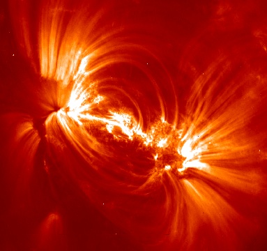
The input image IMAGE1, observed with TRACE on 1998 May 19, 22:21 UT, in the wavelength of 171 A is (with a displayed range of x=200-1000 pixels and y=150-850 pixels; the full image is 1024x1024 pixels):

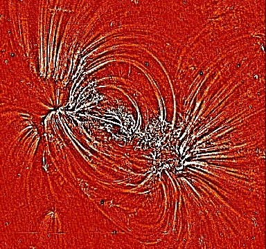
The highpass-filtered IMAGE2, which is provided in the output is (using a smoothing boxcar of NSM=9 in the highpass filter):

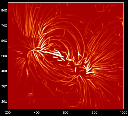
The output produces the x,y-coordinates of the traced loops, stored in the ASCII file LOOPFILE, which can be plotted as follows:

Another representation of the traced loops can be rendered by convolving the (x,y)-coordintes of the traced loops with a 2D Gaussian kernel function scaled to the fluxes (also stored in the datafile LOOPFILE):

The numeric output in the file LOOPFILE looks like this:

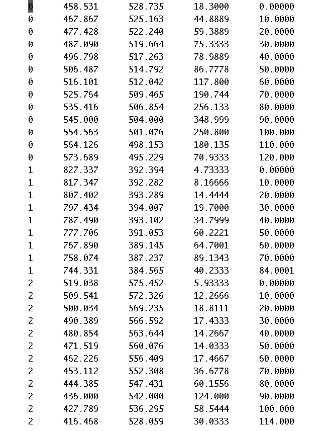
containing the loop number (1st column), the x-coordinates in pixels (2nd column), the y-coordinates in pixels (3rd column), the fluxes in datanumbers per second (DN/s) or whatever the image flux units are (4th column), and the loop length s-coordinate (5th coordinate). This datafile can be read in IDL simply with the procedure READCOL. For a smooth appearance, the loop curves can be interpolated from the spline points given in X and Y with the procedure SPLINE_P, which will produce loop coordinates with about 8 times finer resolution. Of course each loop has to be interpolated separately, for instance:

IDL>..................................................................
READCOL,LOOPFILE,ILOOP,X,Y,Z,S ;read output data
N=MAX(ILOOP)+1 ;maximum loop number
WINDOW,0,XSIZE=800,YSIZE=700
PLOT,[0,0],[0,0],XRANGE=[200,1000],YRANGE=[150,850],XSTYLE=1,YSTYLE=1
LMIN=35
FOR I=0,N-1 DO BEGIN &IND=WHERE(I eq ILOOP,NS) &IF (MAX(S(IND)) ge LMIN) THEN BEGIN &SPLINE_P,X(IND),Y(IND),XX,YY &OPLOT,XX,YY,THICK=3 &ENDIF &ENDFOR
IDL>..................................................................

FITS files of TRACE image examples can be downloaded from here:
http://www.lmsal.com/~aschwand/software/tracing/TRACE_19980519.fits"
http://www.lmsal.com/~aschwand/software/tracing/TRACE_19980825.fits"
http://www.lmsal.com/~aschwand/software/tracing/TRACE_19991106.fits"
http://www.lmsal.com/~aschwand/software/tracing/TRACE_20001109.fits"
http://www.lmsal.com/~aschwand/software/tracing/TRACE_20000714.fits"

(2) EUVI Data Examples

For automated loop tracing one has to be aware that the spatial resolution of the STEREO/EUVI images is about a factor of 3 (1.6 arcsec pixels) lower than for TRACE, so it is recommended to choose the minimum curvature radius of loop (in pixels) as well as the width of loops (in pixels) a corresponding factor lower, so RMIN=40 and WID=3 for TRACE data, but RMIN=13 and WID=1 for EUVI data. Also the flux threshold can be set somewhat lower than NSIG=1, say NSIG=0.5. Some examples of loop tracings in EUVI images are shown in the following plots, where the results are compared with manual tracings (see legend in paper cited above).

FITS files of partial STEREO/EUVI-A images can be downloaded from here:
http://www.lmsal.com/~aschwand/software/tracing/EUVIA_20070430.fits"
http://www.lmsal.com/~aschwand/software/tracing/EUVIA_20070509.fits"
http://www.lmsal.com/~aschwand/software/tracing/EUVIA_20070519.fits"
http://www.lmsal.com/~aschwand/software/tracing/EUVIA_20071211.fits"

The results of the tracings of the 4 EUVI images can be seen here:
http://www.lmsal.com/~aschwand/software/tracing/EUVIA_20070430.gif"
http://www.lmsal.com/~aschwand/software/tracing/EUVIA_20070509.gif"
http://www.lmsal.com/~aschwand/software/tracing/EUVIA_20070519.gif"
http://www.lmsal.com/~aschwand/software/tracing/EUVIA_20071211.gif"

The selected EUVI images and stereoscopically traced loops are described in the following publications:

185) Aschwanden,M.J., Wuelser,J.P., Nitta,N., Lemen,J., and Sandman, A. 2009, The Astrophysical Journal, 695, 12-29
URL1="../eprints/2009_stereo3.pdf" - _movies/"
First 3D reconstructions of coronal loops with the STEREO A and B spacecraft: III. Instant Stereoscopic Tomography of Active Regions

184) DeRosa,M.L., Schrijver,C.J., Barnes,G., Leka,K.D., Lites,B.W., Aschwanden,M.J., Amari,T., Canou,A., McTiernan,J.M., Regnier,S., Thalmann,J., Valori,G., Wheatland,M.S., Wiegelmann,T., Cheung,M.C.M., Conlon,P.A., Fuhrmann,M., Inhester,B., and Tadesse,T. 2009, The Astrophysical Journal, 696, 1780-1791
URL1="../eprints/2009_derosa_nlfff.pdf"
A critical assessment of nonlinear force-free field modeling of the solar corona for active region 10953

181) Sandman,A., Aschwanden,M.J., DeRosa,M., Wuelser,J.P. Alexander,D. 2009, Solar Physics, 259, 1-11
URL1="../eprints/2009_sandman.pdf"
Comparison of STEREO/EUVI Loops with Portential and Force-Free Magnetic Field Models

169) Aschwanden,M.J., Nitta,N.V., Wuelser,J.P., and Lemen,J.R. 2008, The Astrophysical Journal, 680, 1477-1495
URL1="../eprints/2008_stereo2.pdf"
First 3D reconstructions of coronal loops with the STEREO A and B spacecraft: II. Electron Density and Temperature Measurements

167) Aschwanden,M.J., Wuelser,J.P., Nitta,N., and Lemen,J. 2008, The Astrophysical Journal, 679, 827-842
URL1="../eprints/2008_stereo1.pdf" - _loop3D.dat"
First 3D reconstructions of coronal loops with the STEREO A and B spacecraft: I. Geometry

Optimization of Curvi-Linear Tracing Applied to Solar Physics and Biophysics
by M.J.Aschwanden, B. DePontieu, and E. Katrukha (2013), Entropy ... (in preparation).
../eprints/2013_entropy.pdf"

E-mail: aschwanden@lmsal.com - Markus J.Aschwanden (Lockheed Martin Solar & Astrophysics Lab.)