E-mail:
aschwanden@lmsal.com -
Markus J.Aschwanden (Lockheed Martin Solar & Astrophysics Lab.)
- Updated: 24-Jan-2003
HYDROSTATIC CODE - Software Tutorial
This tutorial is intended for SolarSoftWare (SSW) users who want to use
a package of hydrostatic and hydrodynamic codes that calculate numerical
solutions and analytical approximations, based on the paper:
Aschwanden,M.J. and Schrijver,C.J 2002,
The Astrophysical Journal Supplement Series, Vol. 142, p. 269-283
URL1="../eprints/2002_hydro.ps.gz"
Analytical Approximations to Hydrodynamic Solutions and Scaling Laws of Coronal Loops
The IDL procedures of this code should be available in SolarSoft
and have the names:
- HYDRO_ANALYTIC.PRO
- HYDRO_TMAX.PRO
- RADIATIVE_LOSS.PRO
- HYDRO_STATIC.PRO
- HYDRO_NUMERIC.PRO
- HYDRO_NUMERIC_FUNC.PRO
- HYDRO_DISPLAY.PRO
The software package HYDRO can be included in the instrument list $SSW_INSTR (see http://www.lmsal.com/solarsoft/ssw_setup.html) in the start-up file or login file. During the session it can be added with
In the following we give examples that allow to reproduce the examples
shown in the Figures of the paper. The user should be aware of the
restrictions of the valid parameter ranges given in the paper,
for instance all analytical approximations are only tested in the
temperature range of $T=1.0-10.0$ MK, but are probably inaccurate
at cooler temperatures of $T < 1.0$ MK.
Example 1: Analytical Approximation of Hydrostatic Solutions [L, s_H, T_MAX]
Let us calculate the analytical approximation for a hydrostatic solution
for a coronal, semi-circular loop, based on the three independent parameters
[LEN, S_HEAT, T_MAX] :
a loop half length of LEN=20,1000 km,
an exponential heating scale height of S_HEAT=10,000 km,
a looptop maximum temperature TMAX=1 MK,
starting at a coronal loopbase in a height of H_CHR=1300 km where the
base temperature is TMIN=20,000 K.
The routine called is HYDRO_ANALYTIC.PRO.
IDL> TMIN = 2.0e4
.... ;[K] temperature of footpoint in transition region
IDL> TMAX = 1.0e6
.... ;[K] loop top temperature
IDL> LEN = 2.0e9
.... ;[cm] loop half length
IDL> S_HEAT = 1.0e9
.... ;[cm] heating scale height
IDL> H_CHR = 1.3e8
.... ;[cm] height of footpoint in transition region
IDL> NS = 200
.... ;number of loop coordinate points
IDL> S = H_CHR+(LEN-H_CHR)*FINDGEN(NS)/FLOAT(NS-1)
.... ;set up array with loop coordinates
IDL> THETA = 0.
.... ;loop inclination angle
IDL> G_STAR = 1.
.... ;surface gravity of star in unit of solar gravity
IDL> GAMMA = 1.
.... ;geometric loop expansion factor (1=constant cross-section)
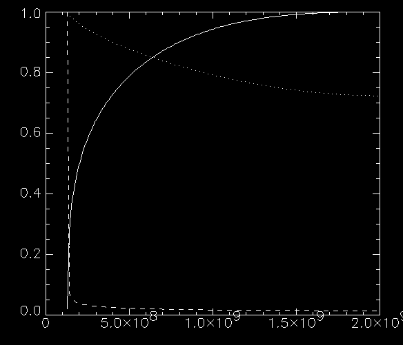
IDL> hydro_analytic,tmin,tmax,s_heat,s,t_s,p_s,n_s,radfunc,radref,eh0,f_s,dptot,etot,a,b
IDL> PLOT, S, T_S/MAX(T_S)
.... ;plot temperature profile
IDL> OPLOT, S, P_S/MAX(P_S), LINESTYLE=1
.... ;plot pressure profile
IDL> OPLOT, S, N_S/MAX(N_S), LINESTYLE=2
.... ;plot density profile
IDL> PRINT, EH0
.... ;heating rate: e.g. E_H0=0.000683 erg cm-s s-1
Example 2: Hydrostatic Solutions for a given Heating Rate [L, s_H, E_H0]
In example [1] the hydrostatic solutions were computed based in the independent
parameters [L, s_H, T_max]. If you wish to prescribe the heating rate E_H0, instead
of the loop top temperature, you can calculate T_MAX from E_H0 first by calling
the procedure HYDRO_TMAX, which just does the inversion of E_H0(T_MAX).
After T_MAX is known, one can proceed the same way as in example [1].
Be aware, that the inversion outside the valid temperature range T=1.0-10.0 MK
will not be accurate.
IDL> EH0=0.000683
.... ;base heating rate in units of [erg cm-s s-1]
IDL> T_MAX = HYDRO_TMAX(EH0, S_HEAT, S)
.... ;calculates T_MAX
IDL> PRINT,T_MAX
.... ;output = loop top temperature [K], e.g. T_MAX=1.0e6
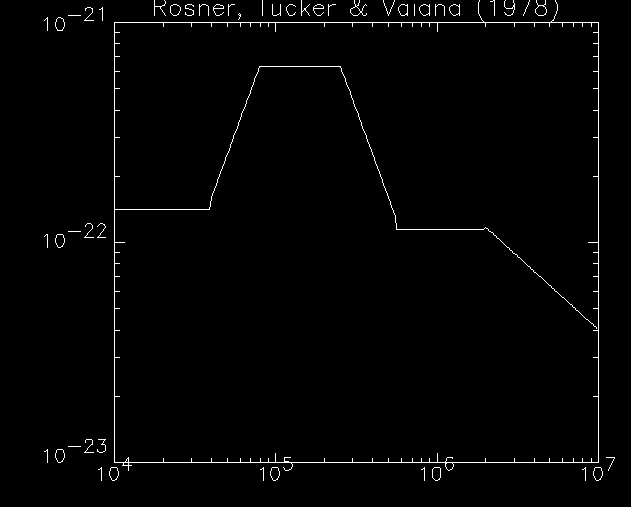
Example 3: Radiative loss function
For the radiative loss function we have 8 variants available.
Choose a code between -2 and +5. The following example demonstrates
the use and shows a plot for the 7-piece powerlaw approximation
by RTV.
IDL> CODE=0
.... ;choose code (0=RTV seven-part power-law approximation
IDL> T = 10.^(4.+0.01*FINDGEN(300))
.... ;temperature array from 10^4 to 10^7 K
IDL> N = FLTARR(300)+1.
.... ;electron density normalized to unity
IDL> E_RAD = RADIATIVE_LOSS(T,N,CODE,REFERENCE)
.... ;
IDL> !P.TITLE=REFERENCE
.... ;
IDL> PLOT_OO,T,-E_RAD
.... ;plot radiative loss function versus temperature
Example 4: Numeric computation of hydrostatic solution
A numeric code to compute a hydrostatic (steady-state) solution for a coronal loop
is provided, which uses a shooting method. The following wrapper routine also
calls the analytical approximation and shows a plot with a comparison of the
numeric with the analytical solution. The numeric values are saved in an
ASCII file.
IDL> len = 1.e10
.... ;[cm] loop half length
IDL> s_heat = 3.e9
.... ;[cm] heating scale length
IDL> tmax = 1.e6
.... ;[K] loop top temperature
IDL> tmin = 2.e4
.... ;[K] loop base temperature
IDL> h_chr = 1.3e8
.... ;[cm] height of loop base
IDL> theta = 0.
.... ;[deg] inclination angle of loop plane
IDL> gamma = 1
.... ;[1...10] loop expansion factor
IDL> radfunc = 0
.... ;[-2,...,5] choice of radiative loss function
IDL> ns = 200
.... ;number of loop coordinate points
IDL> name = 'test'
.... ;name of savefile (*.sav)
IDL> io=0
.... ;output device: 0=screen, 1=ps-file, 2=eps-file, 3=color ps-file
IDL> hydro_static,len,s_heat,tmax,tmin,h_chr,theta,gamma,radfunc,ns,name,io
IDL> $more test.sav
.... ;print savefile

The routine HYDRO_STATIC.PRO calls two different methods, an analytical computation
carried out by HYDRO_ANALYTIC.PRO, and a numeric code HYDRO_NUMERIC.PRO.
An example how both codes are called separately is given here (see also wrapper
routine HYDRO_STATIC.PRO):
IDL> tmin = 2.0e4
.... ;[K] temperature of footpoint in transition region
IDL> tmax = 1.0e6
.... ;[K] loop top temperature
IDL> len = 2.50e8
.... ;[cm] loop half length
IDL> s_heat = 4.00e10
.... ;[cm] heating scale height
IDL> h_chr = 1.30e8
.... ;[cm] height of footpoint in transition region
IDL> ns = 100
.... ;number of loop coordinate points
IDL> s= h_chr+(len-h_chr)*findgen(ns)/float(ns-1)
.... ;array with equidistant loop coordinates (HYDRO_ANALYTIC.PRO)
IDL> p0_start=1.
.... ;start value of iteration of p0 (dyne cm-2)
IDL> e0_start=1.
.... ;start value of iteration of e_h0 (erg cm-3 s-1)
IDL> logmagn=5
.... ;orders of magnitude for range of spatial resolution (at footpoint vs. corona)
IDL> nitmax=100
.... ;maximum limit of iterations
IDL> savefile='hydro_numeric.dat'
.... ;output file name (for routine HYDRO_NUMERIC.PRO)
IDL> silent=0
.... ;no interactive output
IDL> hydro_analytic,tmin,tmax,s_heat,s,t_s,p_s,n_s,radfunc,radref,eh0,f_s,dptot,etot,a,b
.... ;runs analytical code
IDL> hydro_numeric, tmin,tmax,len,s_heat,ns,radfunc,savefile,e0_start,p0_start,logmagn,nitmax,silent
.... ;runs numerical code
IDL> readcol,savefile,s8,t_num,n_num,p_num,f_num,dp_ds,dpgrav,econd,eheat,erad,skipline=13
.... ;reads output from numerical code
IDL> print,'p0 (analytical,numerical)=',p_s(0),p_num(0),' dyne cm-2'
.... ;compare base pressure values between both codes
IDL> print,'eh0 (analytical,numerical)=',eh0 ,eheat(0),' erg cm-2 s-1'
.... ;compare base heating rates between both codes
E-mail:
aschwanden@lmsal.com -
Markus J.Aschwanden (Lockheed Martin Solar & Astrophysics Lab.)