Temperature and Emission Measure Analysis with Automated AIA/SDO Tools (Tutorial)

This tutorial is intended for SolarSoftWare (SSW) users who want to determine differential emission measure (DEM) distributions or temperature and emission measures of coronal structures (active regions, coronal loops) from AIA/SDO data with automated tools. The software is designed for AIA datasets in the 6 coronal wavelengths (131, 171, 193, 211, 335, 94 A). Some features and results of these codes are described in the following paper, on which this tutorial is based on:

Automated Temperature and Emission Measure Analysis of Coronal Loops and Active Regions Observed with AIA/SDO
by M.J. Aschwanden, P. Boerner, R.A. Shine, C.J. Schrijver, and A. Malanushenko (2011), Solar Physics, Topical Issue on "Solar Image Processing in the petabyte Era", Vol. 283, p.5-30
../eprints/2013_autoteem.pdf"

The IDL routines are available in the package $/SSW/packages/mjastereo/idl/, which are automatically included in the IDL path with the command %setenv SSW_INSTR "stereo". Corrections of the AIA response functions of 94 A and 131 A (2012 Feb) and of the DEM code (2014 Oct 22) may slightly change the results displayed on this website (from original paper cited above).

(1) Downloading an AIA 6-wavelength image dataset

For all of the following examples we need an AIA image dataset in the 6 coronal wavelengths. Such a dataset (of 1.0 level processed images) can be downloaded from the AIA/SDO JSOC data archive (see general AIA software documentation) http://www.lmsal.com/sdodocs/). A one-time registration at JSOC is required with your personal EMAIL, and the nofity option with your personal EMAIL is required in subsequent data requests: SSW_JSOC_TIME2DATA,...,NOTIFY="EMAIL". (Please replace Einstein's email address with yours in the example given below.) We write out FITS files for each AIA wavelength and and store it in a local work directory. We select data in a 1-minute time interval and download only the first file in each wavelength, which should include the first 6 coronal wavelength images (during a nominal cadence of 12 s).

IDL>..................................................................
t1 ='15-Feb-2011 00:00'
t2 ='15-Feb-2011 00:01'
wave_ =['94','131','171','193','211','335']
ssw_jsoc_time2data,t1,t2,waves=wave_,index,data,max_files=6,notify='einstein@princeton.edu'
help,index,data
more,get_infox(index,'date_obs,wavelnth,crpix1,crpix2,img_type,datamean')

If the AIA datafiles are accessible from your computer, the output is:
INDEX STRUCT = -> Array[6]
DATA INT = Array[4096, 4096, 6]
2011-02-15T00:00:02.12Z 94 2054.51 2040.19 LIGHT 2.47
2011-02-15T00:00:09.62Z 131 2047.74 2038.45 LIGHT 10.26
2011-02-15T00:00:12.34Z 171 2056.06 2043.72 LIGHT 250.34
2011-02-15T00:00:07.84Z 193 2046.21 2041.09 LIGHT 281.49
2011-02-15T00:00:00.62Z 211 2041.06 2040.20 LIGHT 125.67
2011-02-15T00:00:03.62Z 335 2046.60 2036.76 LIGHT 6.12

We write out FITS files for each wavelengh:
IDL>..................................................................
dir ='~/work_dir/'
fileset ='AIA20110215_0000'
nwave =n_elements(wave_)
data_files=strarr(nwave)
for iw=0,nwave-1 do begin
   data_files(iw)=dir+fileset+'_'+wave_(iw)+'.fits'
   mwritefits,index(iw),data(*,*,iw),outfile=data_files(iw)
   print,'Write FITS file = ',data_files(iw)
endfor
IDL>..................................................................

The name of the FITS files should appear as follows:
Write FITS file = ~/work_dir/AIA20110215_0000_94.fits
Write FITS file = ~/work_dir/AIA20110215_0000_131.fits
Write FITS file = ~/work_dir/AIA20110215_0000_171.fits
Write FITS file = ~/work_dir/AIA20110215_0000_193.fits
Write FITS file = ~/work_dir/AIA20110215_0000_211.fits
Write FITS file = ~/work_dir/AIA20110215_0000_335.fits

(2) AIA Coalignment Test

A first requirement for multi-wavelength studies is a perfect coalignment between the images in different wavelengths. The coalignment of AIA images in the 6 coronal EUV wavelengths is carried out by limb fits and is incorporated in the FITS headers (in the keywords CRPIX1, CRPIX2 that give the pixel number of the Sun center, and RSUN_OBS, DSUN_OBS, and CDELT1, which give the solar radius, solar distance, and the plate scale). The currently reprocessed 1.5-level AIA images have a relative coalignment accuracy of < 1 pixel.

The solar limb in EUV images typically appears a few 1000 km higher than the photospheric altitude level, due to occultation of the bright coronal background by the optically thick chromosphere, which amounts to about 5-10 AIA pixels. We can verify the coalignment accuracy by fitting the EUV limb and verifying the symmetry of the EUV limb offset with respect to the optical limb in east-west and north-south direction. We determine the average radial EUV flux profiles at four positions (east and west limb, south and north pole) and can find the height of the EUV chromosphere in each wavelength by the offset of the location with the steepest flux gradient (supposedly at the top of the chromosphere) from the optical solar radius.

IDL>..................................................................
fileset ='AIA20110215_0000' ; (searchstring for datafiles)
io=0 ; (0=screen, 3=color postscript file)
ct=3 ; (IDL color table)
nsig=3 ; (contrast in number of standard deviations)
nsm=7 ; (smoothing boxcar of limb profiles)
aia_coalign_test,fileset,wave_,io,ct,nsig,nsm,h_km,dx,dy
IDL>..................................................................

The procedure AIA_COALIGN_TEST.pro produces an output on the screen (if you set io=0) or in a color postscript file (if you set io=3), with the filename AIA20110215_0000_coalign_test_col.ps. The output parameters h_km(4,6) contain the chromospheric height measured in the 4 limb positions and 6 wavelengths. The parameters dx(2) and dy(2) contain the mean and standard deviations of the relative coalignment accuracy in x-direction (EW) and y-direction (NS), assuming that the chromospheric heights are symmetric on opposite limb positions. For the present example we find the following output (the coalignment accuracy may change slightly with each reprocessing of the data):

Chromospheric height 131 : 2575 + 429 km
Chromospheric height 171 : 3425 + 650 km
Chromospheric height 193 : 3650 + 974 km
Chromospheric height 211 : 3325 +1172 km
Chromospheric height 335 : 4075 +1347 km
Chromospheric height 94 : 2325 + 525 km
Coalignment in x-direction = 0.99 + 0.63 pixels
Coalignment in y-direction = 0.38 + 0.31 pixels

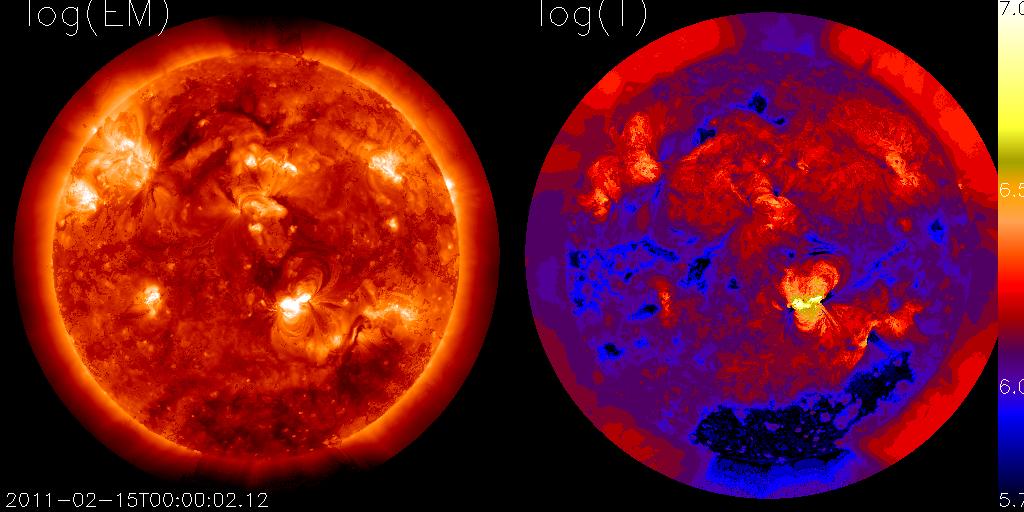
(3) Automated DEM Peak Emission Measure and Peak Temperature Maps

To visualize the emission measures and temperatures in AIA images we fit a DEM solution in each pixel (or macropixel), which can be parameterized by a single Gaussian function that has 3 free parameters: the peak emission measure EM_p(x,y), the peak temperature T_p(x,y), and the temperature width sigma_T(x,y). In our automated code we calculate first a DEM lookup table with the routine AIA_TEEM_TABLE.PRO, for a suitable set of free parameters, which needs to be calculated only once. The current version allows also to use a correction factor for the low-temperature response of the 94 A channel. After that we can obtain EM-maps and T-maps for any arbitrary fileset of 6 AIA filter images with the routine AIA_TEEM_MAP.PRO, either for the full image or partial images. The display of a temperature map can be done with the routine AIA_TEEM_DISP.PRO. Here is an example (using the parameters wave_,io,t1 defined above):

IDL>..................................................................
fileset ='AIA20110215_0000' ; (searchstring for datafiles)
te_range=[0.5,20]*1.e6 ; ([K], valid temperature range for DEM solutions)
tsig=0.1*(1+1*findgen(10)) ; (values of Gaussian logarithmic temperature widths)
q94=1.0 ; (correction factor for low-temperature 94 A response)
fov=[-1,-1,1,1]*1.15 ; (field-of-view [x1,y1,x2,y2] in solar radii)
npix=8 ; (macropixel size=8x8 pixels, yields 512x512 map)
vers='a' ; (version number of label in filenames used for full images)
teem_table='teem_table.sav' ; (savefile that contains DEM loopup table)
teem_map =fileset+vers+'_teem_map.sav' ; (savefile that contains EM and Te maps)
teem_jpeg=fileset+vers+'_teem_map.jpg' ; (jpg-file that shows EM and Te maps)
aia_teem_table2,data_files,wave_,tsig,te_range,q94,teem_table
aia_teem_map2,data_files,fov,wave_,npix,teem_table,teem_map
aia_teem_disp2,teem_map,te_range,t1,teem_jpeg
IDL>..................................................................

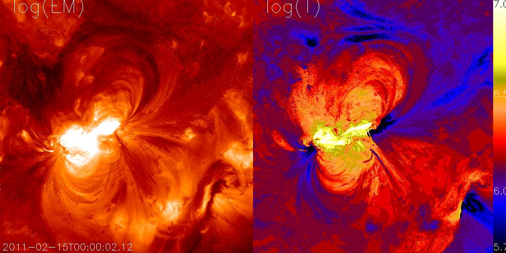
If you want to calculate an EM and Te map of a particular active region with higher spatial resolution, you just define the corresponding field-of-view (fov) in units of solar radii, macropixel size (npix), and give a different version (vers='b') to distinguish the files. The choice of a meaningful field-of-view can be automated too, of course, from local emission measure peaks in the previous total image EM map. Here we give an example by zooming in into AR 1158 that produced the X2.2 flare:

IDL>..................................................................
fov=[-0.03,-0.52,0.60,0.11] ; (field-of-view [x1,y1,x2,y2] of AR 1158)
npix=2 ; (macropixel size=2x2 pixels, yields 512x512 map)
vers='b' ; (version number or label in filenames used for AR 1158)
teem_map =fileset+vers+'_teem_map.sav' ; (savefile that contains EM and Te maps)
teem_jpeg=fileset+vers+'_teem_map.jpg' ; (jpg-file that shows EM and Te maps)
aia_teem_map2,data_files,fov,wave_,npix,teem_table,teem_map
aia_teem_disp2,teem_map,te_range,t1,teem_jpeg
IDL>..................................................................

(4) Total DEM Distribution of an Active Region

The total DEM distribution of an AR can be obtained by summing up the single-Gaussian DEMs of every macropixel, previously calculated with the routine AIA_TEEM_MAP.PRO. The following call of AIA_TEEM_TOTAL.PRO reads the EM and Te savefile (teem_map) and displays the total DEM, stored also in the output savefile (teem_tot). The procedure displays also the observed and theoretically predicted 6 AIA filter fluxes (based on the reconstructed total DEM distribution).

IDL>..................................................................
aia_teem_total2,fileset,fov,npix,wave_,q94,teem_table,vers,mask=mask
IDL>..................................................................

(5) Manual Loop Tracing

Tracing of an individual loop can be done with the routine AIA_LOOP_MANU.PRO. The routine displays a selected fiedl-of-view (FOV) and prompts for the number of loops and

IDL>..................................................................
iwave=1 ; (0,1,2,3,4,5 = number of wavelength filter for tracing)
nsig=3 ; (number of standard deviations to display flux contrast)
aia_loop_manu,fileset,wave_,iwave,fov,vers,nsig
IDL>..................................................................

(6) Automated Loop Tracing

For automated DEM analysis of loops we start with an algorithm that does automated tracing of loop segments that are contiguous and have large curvature radii (OCCULT code). The following procedure AIA_LOOP_AUTO.PRO executes such automated loop tracings in a AIA dataset of 6 filter images in a given field-of-view (fov) and stores the (x,y)-coordinates of the traced loops in a datafile (*.dat), as well as the highpass-filtered images (*F.fits).

IDL>..................................................................
vers='c' ; (label in filename)
fov=[0.00,-0.45,0.45,-0.10] ; (field-of-view [x1,y1,x2,y2] in solar radii)
rmin=25 ; (minimum curvature radius of loop in pixels)
wid=3 ; (typical half width of loop in pixels)
nsig=1.0 ; (threshold level in flux standard deviations)
qfill=0.35 ; (minimum filling factor of traced structure)
reso=10 ; (output resolution of traced loops in pixels)
n=10000 ; (maximum limit of traced structures)
test=n+1 ; (minimum number of traced loop structure)
cutoff=0.01 ; (minimum loop length in solar radii)
para=[rmin,wid,nsig,qfill,reso,n]
aia_loop_auto,fileset,wave_,fov,para,test,cutoff,vers
IDL>..................................................................

A combined view of the loop tracings in all 6 AIA filters can be displayed from a highpass-filtered image (*F.fits) and the loop coordinates in the datafiles (*131.dat, ..., *94.dat):

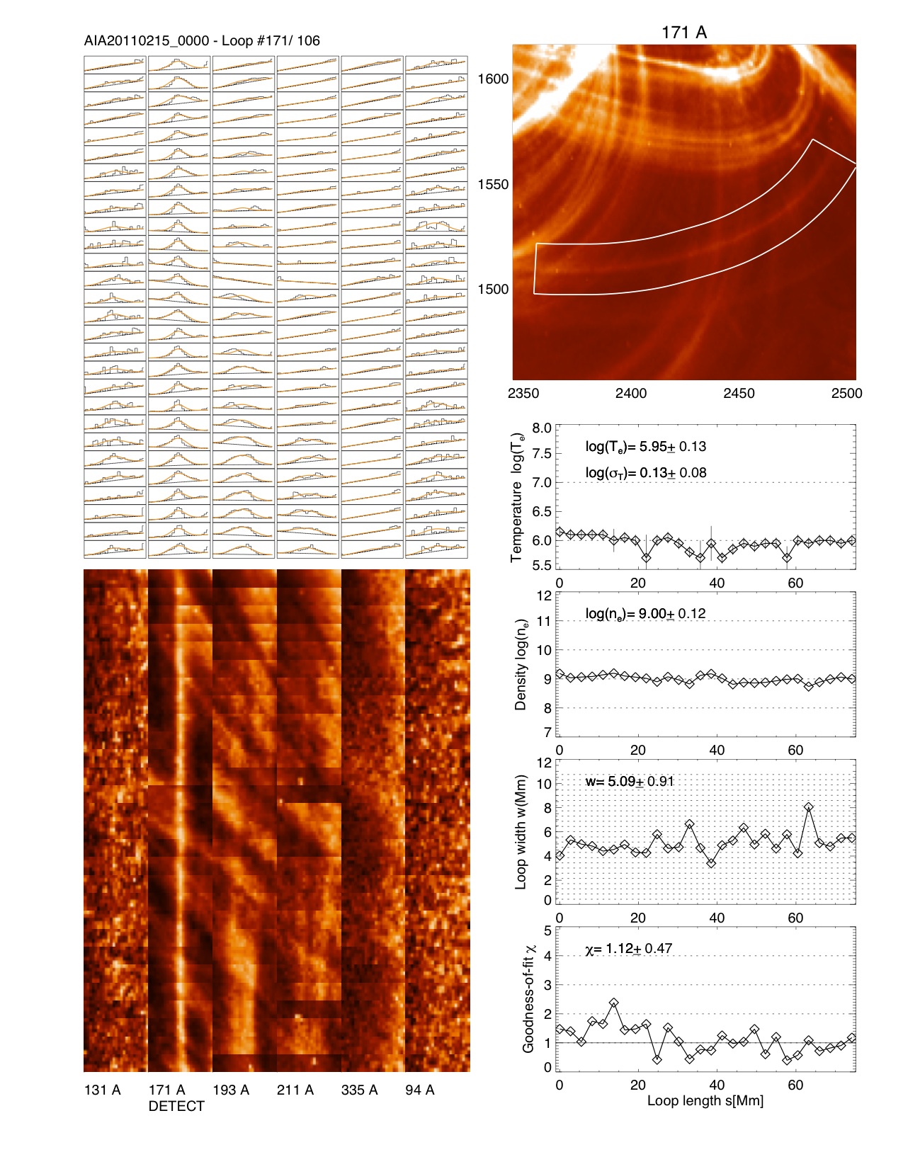
(7) Automated EM and Te Analysis of Coronal Loops

In a next step we break the automatically traced loop segments (570 segments in this example) into chunks with a small length (e.g., ns_step=5 pixels, which yields 3837 locations along the loop segments), and average the cross-sectional loop profiles (with width nw=25 pixels) over this length, apply a DEM forward-fit of the background-subtracted loop fluxes, using the DEM lookup table produced earlier. The procedure AIA_LOOP_AUTODEM.PRO performs these tasks sequentially for all (570) loop segments and we could display the results interactively by choosing segmin=0.01 (minimum length of loop segment in solar radii). However, if we do not have the patience to go through each segment, we can display interactively only those with some larger lengths, say segmin=0.1. After each display, the user can choose to continue, make a postscript file, or to quit the program. All EM and Te parameters of each loop positions are also stored in a savefile (*_teem_cube.sav).

IDL>..................................................................
ns_step=5 ; (number of loop points to integrate along loop)
nw=25 ; (loop cross-sectional width in pixels)
segmin=0.1; (minimum loop length in solar units to display)
vers='a' ; (version label)
chimax=2.0; (upper limit of acceptable chi-square)
test=0 ; (1=display of fits to each loop cross-section)
cubefile =fileset+vers+'_teem_cube.sav' ; (name of savefile for loop EM and Te values)
aia_loop_autodem,fileset,wave_,fov,ns_step,nw,segmin,vers,teem_table,chimax,test
IDL>..................................................................

One example of an interactive display of a loop segment with automated EM and Te analysis looks like this:

(8) Statistics of EM and Te Analysis of Coronal Loops

Statistics of the automatically determined temperatures, temperature widths, electron densities, and loop widths can be displayed in form of histograms with the procedure AIA_LOOP_AUTODISP.PRO, which reads the data stored in the savefile (cubefile). An acceptance limit for the goodness-of-fit chi-square can be set to select only good DEM solutions. A postscript file (aia_loop_autodisp.ps) is generated by setting io=1.

IDL>..................................................................
aia_loop_autodisp,cubefile,te_range,chimax,io
IDL>..................................................................

E-mail: aschwanden@lmsal.com - Markus J.Aschwanden (Lockheed Martin Solar & Astrophysics Lab.)