(h2) Stereoscopic Height Measurement of Point-like Features

For point-like features (for instance ``moss'' or small-scale loops of the size of one or a few pixels) that are visible in both the STEREO A and B images), the height can be measured from the stereoscopic parallax. The routine EUVI_CORR.PRO allows the user to click on such a structure in image A and B, and then calculates the stereoscopic height from the centroid determined in a 3x3 pixel neighborhood of the points.

Let us assume the user has produced a coaligned pair of stereoscopic images in array IMAGE_PAIR[2, NX, NY] and the image parameters are in the variable PARA, both stored in the savefile 'loop_A.sav'. We will store the 3D coordinates of the moss feature in the file 'moss_A.dat':

IDL>
savefile='loop_A.sav'
restore,savefile ;restore saved data from step (2a)
nsm =3 ;smoothing boxcar for highpass filter
fov_moss=[710,850,750,910] ;field-of-view in pixels [i1,j1,i2,j2]
dcont =5 ;contour level step for logarithmic contours LEVEL=DCONT * 2^N
mossfile='moss_A.dat' ;output filename where 3D coordinates of loops are stored
ct =3 ;contour level step for logarithmic contours LEVEL=DCONT * 2^N
euvi_corr,image_pair,para,nsm,fov_moss,dcont,mossfile,ct

The output on the screen will look like this:



After the user clicked a feature in image A (right), the estimated position is projected onto image B (left), with a cross, and the user can click on the peak location of the corresponding feature in image B. The program determines the centroids of the 3x3 pixel neighborhoods (marked with red squares) by a parabolic fit (see display with parabolic fit in window 1).

The output in window 1 will look like this:



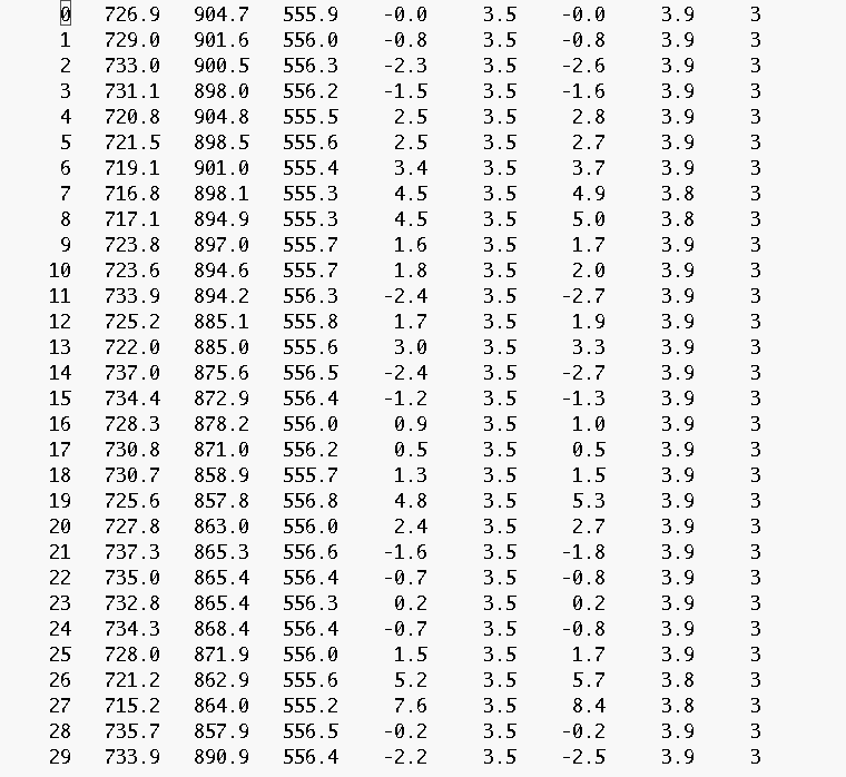
The calculated height is then displayed and the user can decide to save this value in the datafile "moss_A.dat". The procedure can be repeated for an arbitrary number of features, which can subsequently be appended to the same datafile "moss_A.dat". Let us assume you have identified 30 moss features and saved the data in the file "moss_A.dat", which could look like this:



In order to create a summary plot in the context of the entire FOV of the active region we can call:

IDL>
fov =[640,820,800,980] ;field-of-view in pixels [i1,j1,i2,j2]
euvi_corrplot,image_pair,para,nsm,fov_moss,dcont,mossfile,ct,fov

The output on the screen will look like this:



A postscript file will be created with the name corrplot_a_col.ps