(f2) Projection of 3D Coordinates in Arbitrary Direction

Now we want to project the previously obtained 3D coordinates of a set of curvilinear features (e.g., loops or filaments) into an arbitrary direction. Let us suppose you have saved the 3D coordinates in the output file "loop_A.dat", and the images and its parameters are saved in the savefile "loop_A.sav" (as described in task c2). First we want to show it in the projection along the line-of-sight as observed from spacecraft A, which is the reference direction. It has the Sun center position at a relative heliographic longitude BLONG=0, a relative heliographic latitude BLAT=0., and rotation angle CROTA2=0.

IDL>
loopfile ='loop_A.dat' ;output filename where 3D coordinates of loops are stored
savefile='loop_A.sav'
restore,savefile ;restore saved data from step (2a)
crota2 =0. ;rotation angle relative to STEREO-A image (in direction of solar position angle)
blong =0. ;longitude difference relative to STEREO-A image
blat =0. ;latitude difference relative to STEREO-A image
dlat =1. ;spacing of coordinate grid (e.g. 1 deg)
ct =5 ;IDL color scale
h_error =1 ;0=default, 1=with error bars of altitude
hmax =0.1 ;e.g., hmax=0.1 solar radii (maximum height)
window =0 ;IDL window
plotname ='loop_A_proj1' ;plot filename
nops =0 ;produces postscript file (nops=0) or not (nops=-1)
euvi_projection,loopfile,para,crota2,blong,blat,dlat,ct,h_error,hmax,window,plotname,nops

The output on the screen will look like the following. The color varies with the loop numeration.



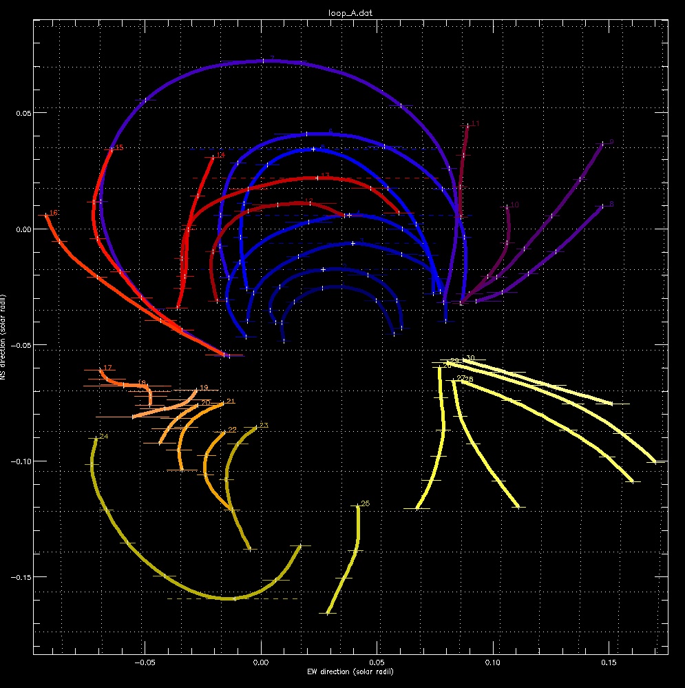
The center of the active region is about 30 deg east of Sun center. So if you want to look straight down in vertical direction, we rotate the 3D coordinates to BLONG=-30:
blong =-30. ;longitude difference relative to STEREO-A image
plotname ='loop_A_proj2' ;plot filename
euvi_projection,loopfile,para,crota2,blong,blat,dlat,ct,h_error,hmax
You will find also a postscript file = projection_a_col.ps created.

The output on the screen will look like this:



Now we would like to visualize the active region side-on, say looking from a southern viewpoint in northern direction, so that the loops appear above the northern horizon. So we keep the (relative) heliographic longitude BLONG=-30 deg as in the previous image, but rotate the line-of-sight by BLAT=90 deg to the northern position:
blong =-30. ;longitude difference relative to STEREO-A image
blat =90. ;latitude difference relative to STEREO-A image
plotname ='loop_A_proj3' ;plot filename
euvi_projection,loopfile,para,crota2,blong,blat,dlat,ct,h_error,hmax


The output on the screen will look like this:



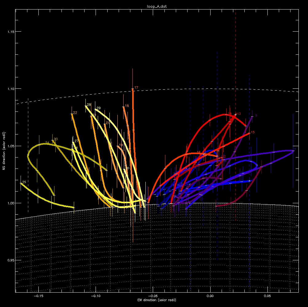
As a last view we want to visualize the inclination angles of the loop plane, so we rotate the active region to the East limb by BLONG=+60 deg, and rotate it by a position angle CROTA2=90 to that the horizon looks horizontally.
blong =+60. ;longitude difference relative to STEREO-A image
blat =0. ;latitude difference relative to STEREO-A image
crota2 =-90. ;relative rotation angle (positive is in anticlock wise direction)
plotname ='loop_A_proj4' ;plot filename
euvi_projection,loopfile,para,crota2,blong,blat,dlat,ct,h_error,hmax


The output on the screen will look like this: