(c2) Stereoscopic 3D reconstruction of a curvi-linear feature

Now we are getting into real stereoscopy, the reconstruction of the 3D geometry of a curvi-linear feature that is visible in a pair or coaligned STEREO images. What we mean with a curvi-linear feature is a one-dimensional structure with arbitrary curvature. It does not neet to be a strictly 1D (and thus unresolved) structure in the mathematical sense, as long as a 1D structure can be uniquely localized in both images, either by an edge or by its cross-sectional centroid. In practice, such curvi-linear futures could be coronal loops or filaments, either directly detectable in the EUV images or in their highpass-filtered versions. The IDL procedure EUVI_STEREO.PRO will use a highpass-filter (defined by the variable NSM=3 [or 5, 7, ...] which defines the smoothing variable of the subtracted smoothed image) to enhance curvi-linear features. The routine then allows a manual input of some spline points of a curve in image A, performs a spline interpolation and transforms its coordinates to image B for an altitude of h=0 and hmax (e.g. = 0.1 solar radii). This visualizes the parallax effect in image B for this height range h=[0,hmax]. The actual coordinates of the loop have then also to be input in image B, usually inside the physical solution range h=[0,hmax]. From the measured offset, the 3D loop coordinates are then computed and stored in the file LOOPFILE. The procedure can be repeated for an arbitrary number of loops, and the 3D coordinates will be appended in the file LOOPFILE. Erroneous entries can also be edited out in the LOOPFILE.

Let us assume you have already done the image coalignment (a2) and tested its accuracy (b2), so that the data in IMAGE_PAIR and PARA can be restored from the savefile.

IDL>
savefile='loop_A.sav'
loopfile ='loop_A.dat' ;output filename where 3D coordinates of loops are stored
nsm =3 ;nsm=3, 5, ..., smoothing boxcar for highpass filtering
fov =[640,820,800,980] ;i1,j1,i2,j2 coordinates of field-of-view
poly =2 ;poly=2, degree of polynom for fitting heights h(s)
hmax =0.1 ;e.g. hmax=0.1 or 0.5 solar radii (maximum height range)
filter =1 ;0=no filter, 1=highpass filter
window =0 ;IDL display window
ct =1 ;IDL color table
wave ='171' ;wavelength '171', '195',' 284', '304'
gamma =1. ;slope of color scale
inv =0 ;0=straight color scale, -1=invert IDL color table
restore,savefile ;restore saved data from step (2a)
euvi_stereo,image_pair,para,nsm,fov,poly,hmax,loopfile,filter,window,ct,wave,gamma,inv



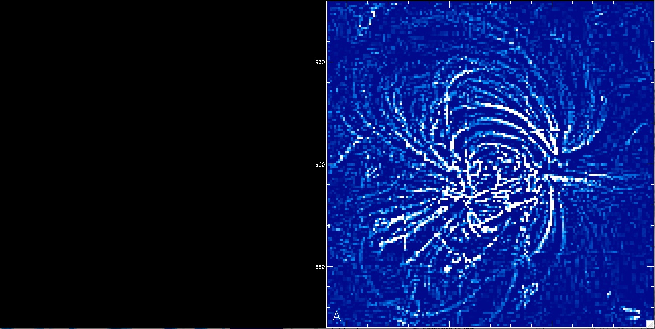
The program prompts you now to narrow down the optimum field-of-view that encompasses an individual loop for stereoscopical triangulation. Click on the bottom-left and top-right corner of the desired enlarged field-of-view.



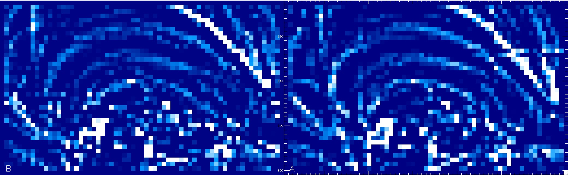
You selected a snug area around a central loop, which is now displayed enlarged for both the spacecraft A and B image. You are now prompted to click a number of say 5-8 loop positions in image A (right). You end the sequence by clicking onto the empty field above image A.

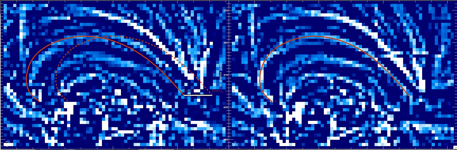The progam switches now to image B and displays the projected coordinates of the loop (red) at a lower height of h=0 and a maximum height of h=hmax (e.g., 0.1 solar radii). The projected height range of every loop position is high-lighted with a black-white bar and you click the corresponding height position for each loop position in image B.

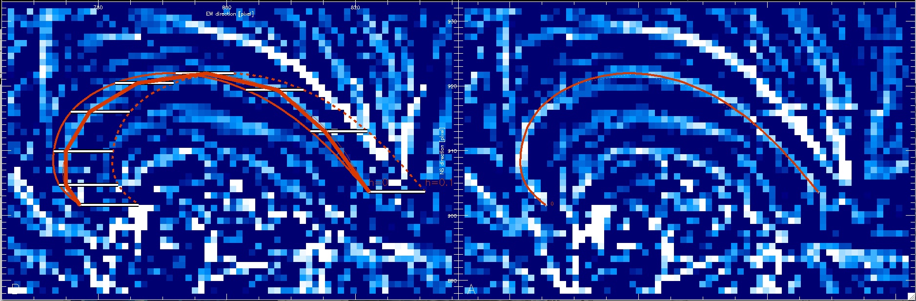After finishing all points of a loop you are asked whether you want to save these loop coordinates. If you are happy you answer with yes and the spline point coordinates are stored in the file loop_A.dat, or discarded else. You can now repeat the whole procedure for every loop and should always get an updated display of the previously traced loops. You can interrupt or resume additional tracing of loops ad infinitum. If you have some stored some bad choices of loop coordinates in the file loop_A.dat, you can edit them out manually.

Once you save the loop coordinates, they will be written into the outputfile "loop_A.dat". The content of the file will look like this, containing 6 lines for each of the 6 loop spline points, where the columns contain: (1) loop identification number, (2) x-pixel (in image A), (3) y-pixel (in image A), (4) z-coordinate (in pixels), (5) the polygon-fitted height (in pixels), (6) the raw values of the stereoscopically correlated height (in pixels), (7) the error of the stereoscopic height measurement (in pixels), (8) the smoothing constant NSM, (9) the degree of the polygon POLY, (10) the chi-square of the polygon height fit, (11) the quality factor of loop A (fraction of pixels along the loop that have a peak at the tracing ridge), and (12) the quality factor of loop B:



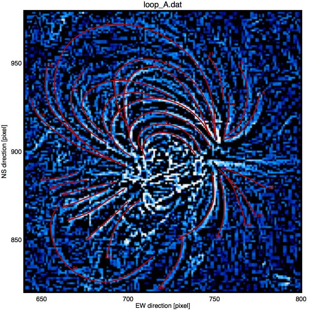
You can now repeat the loop tracing by repeated calling of the routine EUVI_STEREO.PRO and the 3D coordinates will be appended each time into your datafile loop_A.dat. Whenever you trace a new loop in the same image pair, the program first overplots the old loops for your orientation. For example, after 30 traced loops the display may look like this:



The 3D coordinates of the loop spline points are interpolated with higher resolution with the routine EUVI_LOOPFILE.PRO and listed in the file "loop_A2.dat", with [x,y,z] in units of solar radii with respect to Sun center:
tablefile='table2.dat' ;(output for Table 2 in paper Aschwanden et al. 2008 given below)
loopfile2='loop_A2.dat' ;file with interpolated loop 3D coordinates
euvi_loopfile,savefile,loopfile,tablefile,loopfile2

The output file "loop_2A.dat" has 7 columns, containing: (1) loop identification number, (2) loop point position number i, (3) x_i coordinate, (4) y_i coordinate, and (5) z_i coordinate (in solar radii with respect from Sun center), (6) loop length coordinate s_i (in units of Mm), and (7) altitude h_i. The output for the first loop is:



For a full documentation of this example see the publication:
Aschwanden,M.J., Wuelser,J.P., Nitta,N., and Lemen,J. 2008, (ApJ)
URL1="../../eprints/2008_stereo.pdf"
First 3D reconstruction of coronal loops with the STEREO A+B spacecraft: I. Geometry